
, I discussed how to create your first DataFrame using Pandas. I mentioned that the first thing you need to master is Data structures and arrays before moving on to data analysis with Python.
Pandas is an excellent library for data manipulation and retrieval. Combine it with Numpy and Seaborne, and you’ve got yourself a powerhouse for data analysis.
In this article, I’ll be walking you through practical ways to filter data in pandas, starting with simple conditions and moving on to powerful methods like .isin(), .str.startswith(), and .query(). By the end, you’ll have a toolkit of filtering techniques you can apply to any dataset.
Without further ado, let’s get into it!
Importing our data
Ok, to start, I’ll import our pandas library
# importing the pandas library
import pandas as pd
That’s the only library I’ll need for this use case
Next, I’ll import the dataset. The dataset comes from ChatGPT, btw. It consists of basic sales transaction records. Let’s take a look at our dataset.
# checking out our data
df_sales = pd.read_csv('sales_data.csv')
df_sales
Here’s a preview of the data

It consists of basic sales records with columns OrderId, Customer, Product, Category, Quantity, Price, OrderDate and Region.
Alright, let’s begin our filtering!
Filtering by a single condition
Let’s try to select all records from a particular category. For instance, I want to know how many unique orders were made in the Electronics category. To do that, it’s pretty straightforward
# Filter by a single condition
# Example: All orders from the “Electronics” category.
df_sales[‘Category’] == ‘Electronics’
In Python, you need to distinguish between the = operator and the == operator.
= is used to assign a value to a variable.
For instance
x = 10 # Assigns the value 10 to the variable x== on the other hand is used to compare two values together. For instance
a = 3
b = 3
print(a == b) # Output: True

c = 5
d = 10
print(c == d) # Output: False
With that said, let’s apply the same notion to the filtering I did above
# Filter by a single condition
# Example: All orders from the “Electronics” category.
df_sales[‘Category’] == ‘Electronics’
Here, I’m basically telling Python to search through our entire record to find a category named Electronics. When it finds a match, it displays a Boolean result, True or False. Here’s the result

As you can see. We are getting a Boolean output. True means Electronics exists, while False means the latter. This is okay and all, but it can become confusing if you’re dealing with a large number of records. Let’s fix that.
# Filter by a single condition
# Example: All orders from the “Electronics” category.
df_sales[df_sales[‘Category’] == ‘Electronics’]
Here, I just wrapped the condition in the DataFrame. And with that, we get this output

Much better, right? Let’s move on
Filter rows by numeric condition
Let’s try to retrieve records where the order quantity is greater than 2. It’s pretty straightforward.
# Filter rows by numeric condition
# Example: Orders where Quantity > 2
df_sales[‘Quantity’] > 2
Here, I’m using the greater than > operator. Similar to our output above, we’re gonna get a Boolean result with True and False values. Let’s fix it up real quick.

And there we go!
Filter by date condition
Filtering by date is straightforward. For instance.
# Filter by date condition
# Example: Orders placed after “2023–01–08”
df_sales[df_sales[“OrderDate”] > “2023–01–08”]
This checks for orders placed after January 8, 2023. And here’s the output.

The cool thing about Pandas is that it converts string data types to dates automatically. In cases where you encounter an error. You might want to convert to a date before filtering using the to_datetime() function. Here’s an example
df[“OrderDate”] = pd.to_datetime(df[“OrderDate”])This converts our OrderDate column to a date data type. Let’s kick things up a notch.
Filtering by Multiple Conditions (AND, OR, NOT)
Pandas enables us to filter on multiple conditions using logical operators. However, these operators are different from Python’s built-in operators like (and, or, not). Here are the logical operators you’ll be working with the most
& (Logical AND)
The ampersand (&) symbol represents AND in pandas. We use this when we’re trying to fulfil two conditions. In this case, both conditions have to be true. For instance, let’s retrieve orders from the “Furniture” category where Price > 500.
# Multiple conditions (AND)
# Example: Orders from “Furniture” where Price > 500
df_sales[(df_sales[“Category”] == “Furniture”) & (df_sales[“Price”] > 500)]
Let’s break this down. Here, we have two conditions. One that retrieves orders in the Furniture category and another that filters for prices > 500. Using the &, we’re able to combine both conditions.
Here’s the result.

One record was managed to be retrieved. Looking at it, it meets our condition. Let’s do the same for OR
| (Logical OR)
The |,vertical bar symbol is used to represent OR in pandas. In this case, at least one of the corresponding elements should be True. For instance, let’s retrieve records with orders from the “North” region OR “East” region.
# Multiple conditions (OR)
# Example: Orders from “North” region OR “East” region.
df_sales[(df_sales[“Region”] == “North”) | (df_sales[“Region”] == “East”)]
Here’s the output

Filter with isin()
Let’s say I want to retrieve orders from multiple customers. I could always use the & operator. For instance
df_sales[(df_sales[‘Customer’] == ‘Alice’) | (df_sales[‘Customer’] == ‘Charlie’)]Output:

Nothing wrong with that. But there’s a better and easier way to do this. That’s by using the isin() function. Here’s how it works
# Orders from customers ["Alice", "Diana", "James"].
df_sales[df_sales[“Customer”].isin([“Alice”, “Diana”, “James”])]
Output:

The code is much easier and cleaner. Using the isin() function, I can add as many parameters as I want. Let’s move on to some more advanced filtering.
Filter using string matching
One of Pandas’ powerful but underused functions is string matching. It helps a ton in data cleaning tasks when you’re trying to search through patterns in the records in your DataFrame. Similar to the LIKE operator in SQL. For instance, let’s retrieve customers whose name starts with “A”.
# Customers whose name starts with "A".
df_sales[df_sales[“Customer”].str.startswith(“A”)]
Output:

Pandas gives you the .str accessor to use string functions. Here’s another example
# Products ending with “top” (e.g., Laptop).
df_sales[df_sales[“Product”].str.endswith(“top”)]
Output:

Filter using query() method
If you’re coming from a SQL background, this method would be so helpful for you. Let’s try to retrieve orders from the electronics category where the quantity > 2. It can always go like this.
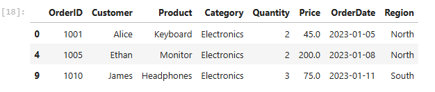
df_sales[(df_sales[“Category”] == “Electronics”) & (df_sales[“Quantity”] >= 2)]Output:
But if you’re someone trying to bring in your SQL sauce. This will work for you instead
df.query(“Category == ‘Electronics’ and Quantity >= 2”)You’ll get the same output above. Pretty similar to SQL if you ask me, and you’ll be able to ditch the & symbol. I’m gonna be using this method quite often.
Filter by column values in a range
Pandas allows you to retrieve a range of values. For instance, Orders where the Price is between 50 and 500 would go like this
# Orders where the Price is between 50 and 500
df_sales[df_sales[“Price”].between(50, 500)]
Output:

Pretty straightforward.
Filter missing values (NaN)
This is probably the most helpful function because, as a data analyst, one of the data cleaning tasks you’ll be working on the most is filtering out missing values. To do this in Pandas is straightforward. That’s by using the notna() function. Let’s filter rows where Price is not null.
# filter rows where Price is not null.
df_sales[df_sales[“Price”].notna()]
Output:

And there you go. I don’t really notice the difference, though, but I’m gonna trust it’s done.
Conclusion
The next time you open a messy CSV and wonder “Where do I even start?”, try filtering first. It’s the quickest way to cut through the noise and find the story hidden in your data.
The transition to Python for data analysis used to feel like a huge step, coming from a SQL background. But for some reason, Pandas seems way easier and less time-consuming for me for filtering data
The cool part about this is that these same techniques work no matter the dataset — sales numbers, survey responses, web analytics, you name it.
I hope you found this article helpful.
I write these articles as a way to test and strengthen my own understanding of technical concepts — and to share what I’m learning with others who might be on the same path. Feel free to share with others. Let’s learn and grow together. Cheers!
Feel free to say hi on any of these platforms